Solving Naive Bayes By Hand

This is part two in a series on classification with Naive Bayes.

Learning Naive Bayes Through Repeated Interceptions

On the whole, the Naive Bayes class of algorithms tends to be pretty easy to understand, which is a part of that class’s popularity. So let’s see how easy it really is by solving a problem with Naive Bayes.

The 2018 NFL season is officially over (playoffs? What are those?) so let’s take a look at a team which is most glad the Cleveland Browns exist so that they don’t get all of the smack talk: the Buffalo Bills.

This year, the Bills went 6-10. I’m going to use Naive Bayes techniques to build a predictor for whether the Bills will lose yet again. This will be useful if ever I spend an eternity having to re-watch the 2018 NFL season; I have already resolved to clean up my life to avoid this fate and I haven’t even built the predictor yet…

To make this easy, I’m going to pick four variables:

• Who was the starting quarterback? My set is { Josh Allen, Somebody Else } as that gives a fairly nice split of 11 games versus 5 games.
• Was this a home game or an away game? My set is { Home, Away } and naturally breaks down 8-8.
• Did the team score at least 14 points? My set is { Yes, No } and sadly, 13-14 points was the median points scored.
• Who was the top Bills receiver in terms of yardage? My potential set is { Zay Jones, Chris Ivory, LeSean McCoy, Charles Clay, Kelvin Benjamin, Robert Foster }. Yep, on three separate occasions, running backs led the team in receiving yardage, and we aren’t talking about elite receiving backs like Alvin Kamara. But I’m not going with that full set because 3 of those 6 top receivers were 100% winners or (generally) 100% losers—I’ll explain why this matters later. So let’s bundle Ivory + McCoy and Clay + Benjamin, leaving Jones and Foster alone.

So with these four variables in mind, we’re going to try to predict whether the Bills would be favored to win or lose a game. Here’s how things stack up:

Game	QB	H/A	14 Points?	Top Receiver	W/L
1	Other	A	N	Zay Jones	L
2	Allen	H	Y	Zay Jones	L
3	Allen	A	Y	Chris Ivory	W
4	Allen	A	N	Charles Clay	L
5	Allen	H	N	LeSean McCoy	W
6	Allen	A	N	Kelvin Benjamin	L
7	Other	A	N	Kelvin Benjamin	L
8	Other	H	N	LeSean McCoy	L
9	Other	H	N	Kelvin Benjamin	L
10	Other	A	Y	Robert Foster	W
11	Allen	H	Y	Robert Foster	W
12	Allen	A	Y	Zay Jones	L
13	Allen	A	Y	Robert Foster	L
14	Allen	H	Y	Robert Foster	W
15	Allen	A	N	Zay Jones	L
16	Allen	H	Y	Zay Jones	W

Now that we have our data, it’s time to solve the problem. At least the problem of predicting victory, not the problem of scoring two touchdowns per game.

Trust the Process

There are three steps to the process of solving the simplest of Naive Bayes algorithms. They are:

1. Find the probability of winning a game (that is, our prior probability).
2. Find the probability of winning given each input variable: whether Josh Allen starts the game, whether the team is home or away, whether the team scores 14 points, and who the top receiver was.
3. Plug in values from our new data into the formula to obtain the posterior probability.

So let’s get to it!

Prior Probability

Our prior probability is the likelihood of a win or a loss independent of any other conditions. The Bills went 6-10, so their probability of a win was 6/16 or 0.375.

Per-Variable Probabilities

Now things get a little busier, but we’ll look at it step by step. We want to get the probability of a victory for each value of each variable independent of all other variables. It sounds complicated but it really isn’t. Let’s see how easy it is with an example.

By Quarterback

QB	W	L	P(W)	P(L)
Allen	5	6	5/6 = .833	6/10 = .600
Other	1	4	1/6 = .167	4/10 = .400
Total:	6	10	100%	100%

Home or Away?

Location	W	L	P(W)	P(L)
Home	4	4	4/6 = .667	4/10 = .400
Away	2	6	2/6 = .333	6/10 = .600
Total:	6	10	100%	100%

Scored 14+ Points?

“Big” Offense	W	L	P(W)	P(L)
14+ Points	5	3	5/6 = .833	3/10 = .300
< 14 Points	1	7	1/6 = .167	7/10 = .700
Total:	6	10	100%	100%

Top Receiver

Top Receiver	W	L	P(W)	P(L)
Clay + Benjamin	0	4	0/6 = .000	4/10 = .400
Ivory + McCoy	2	1	2/6 = .333	1/10 = .100
Robert Foster	3	1	3/6 = .500	1/10 = .100
Zay Jones	1	4	1/6 = .167	4/10 = .400
Total:	6	10	100%	100%

As I mentioned above, I combined some receivers together so that I didn’t end up with 100% probabilities. Well, Clay + Benjamin work well together as “guys the team gave up on and/or vice versa” and I think it’s fitting they belong together. Meanwhile, Ivory & McCoy were the running backs, so there’s something that feels right about combining them. Foster and Jones had both wins and losses so I could leave them be.

Plug In Some Values

We now have our independent probability tables, so we can estimate whether the team will win or lose given these relevant inputs. Our formula for victory is:

We have a formula for victory, but we also need a formula for a loss. Technically a team can tie, but the Bills didn’t have any ties this year, so I’m treating it as a two-class problem to make things easier to follow.

There’s one more thing I need to bring up here: We don’t really know the true probability of our particular set of variables coming true, the P(x) in our examples. But when we’re classifying, we technically don’t need to know P(x) because that part of the formula cancels out when doing an inequality comparison between P(W|x) and P(L|x). This is great for us because it makes our problem tractable, but it comes at the cost that our “probabilities” that we output aren’t truly probabilities, so there’s another step if we really want to get those values.

With those formulas in mind, let’s test some situations.

Scenario 1: The Big Win

I’m going to throw out my ringer lineup here.

• Josh Allen is the starter.
• The team is playing at home.
• The team scores at least 14 points.
• Robert Foster is the leading receiver.

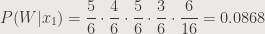
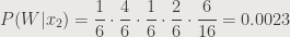
So we plug in the values of our two formulas based on the tables above. Let’s start with winning. With appropriate subscripts we have:

Plugging in values from the table we have our partial probability for victory:

And for a loss:

As you can see, a win is much more likely than a loss in this scenario. As I mentioned above, the two outcomes are not really probabilities (even though I still call it “P”), but we can calculate that the probability of a win is approximately 97% by taking the partial probability of victory (0.0868) and divide by the total pool of partial probabilities (0.0868 + 0.003). Most of the time, though, we don’t need to know the percentages—we just need to know that the Bills are likely to win this game, and it’s not close.

Scenario 2: The Big Push

In this scenario, we’ll change the inputs a little bit:

• Nathan Barkerson is the quarterback.
• The team is still playing at home.
• The team does not score 14 points.
• A running back is the leading receiver.

I won’t do the LaTeX formulas for each step in the process, just the probabilities. Hopefully you get it at this point. Here’s the partial probability of victory:

And again, for a loss:

This is a Buffalo Push: a 75% chance of losing. Speaking of losing…

Scenario 3: The Big Loser

This final scenario will hit on an issue with Naive Bayes that we’ll solve in a future post.

• Josh Allen is the quarterback.
• The team is playing at home.
• The team scores 14 or more points.
• Charles Clay and Kelvin Benjamin fight over the ball like two junkyard dogs, combining for an awe-inspiring 35 yards of receiving between the two of them, with Benjamin’s 18 yards of receiving good enough for first place.

Let’s plug the values into our formula once more, starting with a victory:

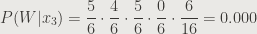
And for a loss:

So this is pretty interesting. The likelihood of victory was looking great, but Benjamin and Clay never led the team in receiving for a victory, so our expected probability of success is 0. Because Naive Bayes has us perform a cross product of these independent probabilities, if one of the component probabilities is 0, the whole thing is 0.

That’s an interesting problem, and one we’ll look at in our next post as I move from predicting Bills victories to classifying words as belonging to particular categories.

Conclusion

In today’s post, we created a Naive Bayes model by hand and populated it with several scenarios. We also discovered that when a component has an outcome probability of 0—particularly common in sparse data sets like the one we have—we can end up with an unexpected result.

In next week’s installment, we will take this algorithm one step further and classify text and figure out this zero-probability outcome problem in the process.