Connecting To Hadoop

Yesterday, we loaded some data sets into Hadoop.  Today, I’m going to show how we can link everything together.  By the end of this blog post, we’re going to have a functional external table which reads from our Second Basemen data set.

Prep Work

We’re going to need to do a little bit of prep work on our SQL Server instance.

External Data Source

First, we will need to create an external data source which points to our Hadoop cluster’s name node.  Because we’re using a Hortonworks sandbox, our name node is the only node, so that makes it easy.  In my case, that IP address is 192.168.172.149.

CREATE EXTERNAL DATA SOURCE [HDP] WITH (TYPE = Hadoop, LOCATION = N'hdfs://192.168.172.149:8020')

I’m calling my external data source HDP (Hortonworks Data Platform) and specifying the type as Hadoop and the location as an HDFS location, using port 8020.  Note that even if we’re connecting to Azure Blob Storage, we will still want to use TYPE = Hadoop.  We’d switch types when connecting to an Elastic Database on Azure.

Also, the Hortonworks sandbox should be open, meaning that you should not need to mess with any firewall settings on that machine.  You might need to mess with firewall settings on your SQL Server instance.  For the sake of simplicity (and because this is a virtual machine that I only turn on for demos), I just turned off the Windows firewall.

Data Type

The next thing we need to do is specify a data type.  When we link an external table, we need to be able to explain, before the link, what structure we expect.  To do that, we’ll create an external file format.

CREATE EXTERNAL FILE FORMAT [CSVTextFileFormat]
WITH (FORMAT_TYPE = DelimitedText, FORMAT_OPTIONS (FIELD_TERMINATOR = N',', USE_TYPE_DEFAULT = True))
GO

This file format is of FORMAT_TYPE DelimitedText, and our delimiter is a comma.  We have a few options available to us.  My recommendation is that, once you get familiar with Polybase, you start looking at other file formats.  ORC and Parquet are optimized for a nice combination of compression and performance, and they tend to be a good bit faster than using simple delimited text files.  Because I want this to be as easy an introduction as possible, I’m sticking with comma-separated value files.

An interesting thing about FIELD_TERMINATOR is that it can be multi-character.  MSDN uses ~|~ as a potential delimiter.  The reason you’d look at a multi-character delimiter is that not all file formats handle quoted identifiers—for example, putting quotation marks around strings that have commas in them to indicate that commas inside quotation marks are punctuation marks rather than field separators—very well.  For example, the default Hive SerDe (Serializer and Deserializer) does not handle quoted identifiers; you can easily grab a different SerDe which does offer quoted identifiers and use it instead, or you can make your delimiter something which is guaranteed not to show up in the file.

You can also set some defaults such as date format, string format, and data compression codec you’re using, but we don’t need those here.  Read the MSDN doc above if you’re interested in digging into that a bit further.

Create An External Table

Now that we have a connection to Hadoop and a valid file format, we can create an external table.  The job of an external table is to represent a Hadoop file or directory as a SQL Server table.  SQL Server is a structured data environment, so we need to provide a structure on top of the file(s) in Hadoop, similar to what we would do in Hive to create a table there.

Here’s the SQL statement to create an external table pointing to our /tmp/ootpoutput/secondbasemen.csv file:

CREATE EXTERNAL TABLE [dbo].[SecondBasemen]
(
	[FirstName] [varchar](50) NULL,
	[LastName] [varchar](50) NULL,
	[Age] [int] NULL,
	[Bats] [varchar](5) NULL,
	[Throws] [varchar](5) NULL
)
WITH
(
	LOCATION = N'/tmp/ootpoutput/SecondBasemen.csv',
	DATA_SOURCE = HDP,
	FILE_FORMAT = CSVTextFileFormat,
	-- Up to 5 rows can have bad values before Polybase returns an error.
	REJECT_TYPE = Value,
	REJECT_VALUE = 5
)
GO

The first half of the CREATE TABLE statement looks very familiar, except that we’re using the keyword EXTERNAL in there.  Note that I’m creating the table in the dbo schema; that’s not required, and you can safely create the table in any schema you’d like.

The second half of the create statement is quite different from our normal expectations, so let’s unpack it one line at a time.  The first line asks where our file or directory is located, and we know that’s at /tmp/ottpoutput/SecondBasemen.csv in HDFS.  We’re pointing at a Hadoop cluster, so take care about case, as things here are case-sensitive.

The next two lines are what we just prepped:  data source and file format.  Our data source is the HDP sandbox, and our file format is a CSV file.  After that, we have two new lines:  REJECT_TYPE and REJECT_VALUE.  REJECT_TYPE has two options:  “Value” or “Percentage” and determines whether to reject after X number of bad rows or a certain percentage of bad rows.  REJECT_VALUE, meanwhile, fills in “X” above.  The idea here is that when we apply structure to a semi-structured data set, we can expect some number of rows to be bad.  Maybe we have a header row in our data file (like in my second basemen example above!), or we didn’t capture all of the data, or maybe we have multiple types of lines in a file—for example, think about a web server log which stores different formats for informational, warning, and error messages—or maybe there was even some kind of corruption or bug in the application.  Regardless of the reason, we can expect that there will be some data which does not quite fit the structure we want to apply, and this gives us a good opportunity to ignore that bad data without throwing exceptions.  You can set REJECT_VALUE = 0 for times in which you absolutely need 100% consistent data, but that does mean that if you get 99% of the way through a hundred million-line file and one bad record exists, the entire query will fail.

For gigantic files, it might help to set REJECT_TYPE to Percentage, REJECT_VALUE to some percentage (e.g., 20.0), and REJECT_SAMPLE_VALUE to a number like 1000 or 10,000.  MSDN explains how the three work together.

Let’s Get Some Data!

Now that we have the external table set up, I want to run three queries.

Basic Check

The first query will be a simple SELECT * from the SecondBasemen table.

SELECT * FROM dbo.SecondBasemen;

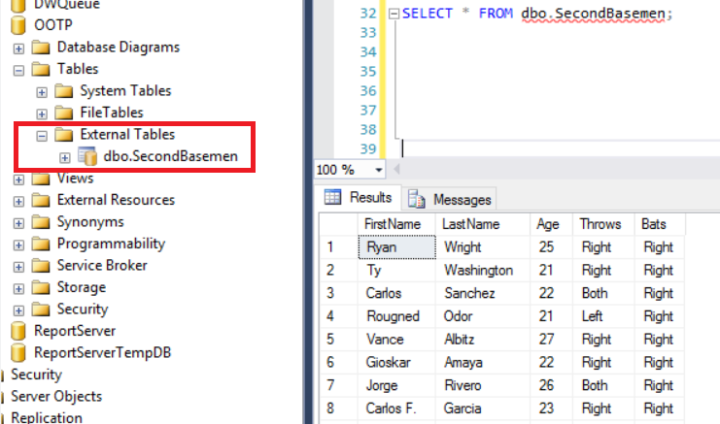
If you’ve followed along, you should get 777 results back.  I also want to note that to see the SecondBasemen table, you go to Tables –> External Tables and you’ll see dbo.SecondBasemen.  For normal purposes, it shows up just like any other table.  You can’t create any key constraints or indexes on it, but you can create statistics, something we’ll talk about later.

The query plan itself is pretty boring: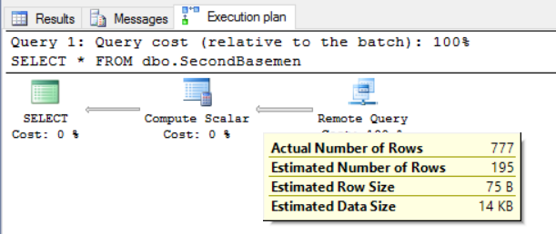

We have a remote query which is responsible for 100% of the query cost.  Then we have a Compute Scalar whose job it is to coerce incoming data into the appropriate format, and that data gets sent to the result set window.

Basic Join

The second query will join to a SQL Server table.  In this case, it’s a tally table, and we join on age.  I could use this to filter ages or filter out players without age information, but in this simple query, I’m just (just?!) joining a T-SQL table to the results of a Polybase query.

SELECT
	sb.FirstName,
	sb.LastName,
	sb.Age,
	sb.Throws,
	sb.Bats
FROM dbo.SecondBasemen sb
	INNER JOIN dbo.Tally t
		ON sb.Age = t.N;

The execution plan looks like you’d expect.  This time, I’m switching to SQL Sentry Plan Explorer to see the whole thing.

This shows that we’re pulling back the 777 rows from the SecondBasemen table and then joining to the Tally table using a nested loop join, returning the results to the user.

Slightly More Complex Query

The third query is a more complex query in which I want to filter out players early.  I’m only looking for players in their prime—that is, between the ages of 26 and 29.  I then join to the tally table, and I include a ROW_NUMBER()  ordered by age, last name, and first name.  Finally, I want to use a CROSS APPLY operation to give just a little more context.  This is all supposed to represent something closer to a realistic query, in which we’re doing multiple things with the data and don’t necessarily want to burn through millions of rows of data just to get out the records we want.

SELECT
	sb.FirstName,
	sb.LastName,
	sb.Age,
	sb.Throws,
	sb.Bats,
	ROW_NUMBER() OVER (ORDER BY sb.Age, sb.LastName, sb.FirstName) AS RowNum,
	tl.TargetLikelihood
FROM dbo.SecondBasemen sb
	INNER JOIN dbo.Tally t
		ON sb.Age = t.N
	CROSS APPLY
	(
		SELECT
			CASE
				WHEN sb.Age <= 28 AND sb.Bats IN ('Left', 'Switch') THEN 'Prime Target' 				WHEN sb.Age > 28 THEN 'Not a Prime Target'
				ELSE 'Medium Target'
			END AS TargetLikelihood
	) tl
WHERE
	sb.Age BETWEEN 26 AND 29
ORDER BY
	tl.TargetLikelihood DESC;

The execution plan gets very interesting, so let’s look at it in some detail.

First, the remote query returns 94 records.  This means that we successfully pushed down the “WHERE sb.Age BETWEEN 26 and 29” to Hadoop.  The query optimizer understood that it would make more sense to do this as a MapReduce job rather than pull back all records and filter using SQL Server’s database engine.  I should note that the optimizer is smart enough to behave the same away even if the filter has WHERE t.N BETWEEN 26 and 29 instead of sb.Age, as that’s part of the join criteria.

Next up, we have a Compute Scalar.  This operation associates our columns, but also gives us the TargetLikelihood expression for free.  Our target likelihood expression represents something like a GM coming to you and saying that he wants to target any lefty-batting (or switch hitting) second basemen between the ages of 26 and 28, but is willing to look at righties if need be.  The first sort operation sorts on Age, LastName, and FirstName, and sets up our window function which provides a numeric order for each batter based on these criteria.  Because we’re sorting by age, we could potentially merge join the results to Tally, but the optimizer (which believes that there are 18 rows at this point) figures that it’s easier to do a nested loop join.  At any rate, once the nested loop join is done, we segment and sequence, which are the hallmarks of a ROW_NUMBER() operation.  Finally, I want to re-sort the data by target likelihood and present it to the end user.

Conclusion

We now have a simple data set hooked up using Polybase.  That’s pretty exciting, and hopefully the three queries above start to give you ideas of what you can do with the data.

Next up, I want to integrate the airline data we added, in order to see how things look once you introduce a larger-scale problem.  We’ll also want to take advantage of Polybase statistics, so I’ll introduce those.

Advertisement